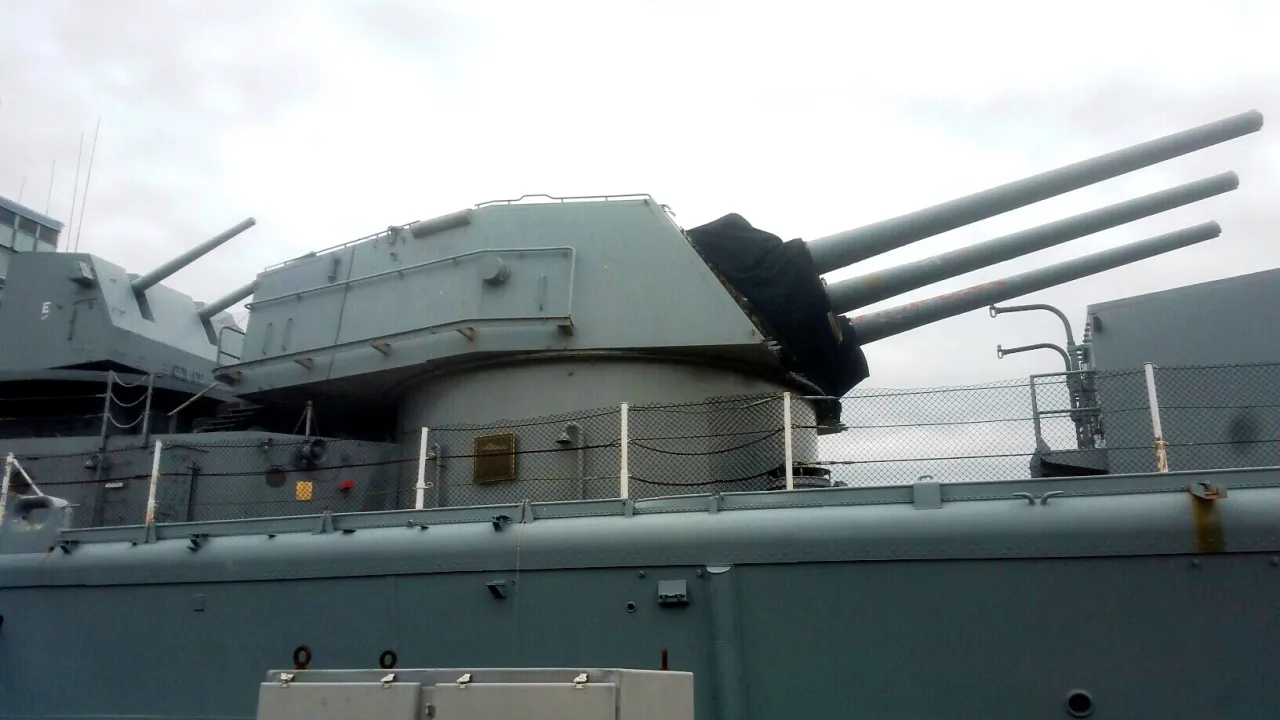
On the problems of the 8-inch/55 guns of the heavy cruiser "Des Moines" when firing at long distances
This article is heavily laden with mathematical calculations, mean deviations, dispersion ellipses, and other tangents. Therefore, for those esteemed readers who don't have the time to delve into all these subtleties, I will immediately present the conclusions.
Unlike the 220mm/65 guns of the Soviet Project 66 cruiser, artillery The De Moines was ill-suited for long-range combat. Due to its ballistic properties and the large vertical dispersion of its shells ("mortar ballistics"), the accuracy of American 203mm/55 guns at ranges of 100 and 150 kbt was approximately 2 and 2,5 times inferior to that of the Soviet 220mm/65 guns, respectively.
For those esteemed readers who have the time and desire to understand the issue, I suggest considering some of the features of long-distance shooting.
Scatter Ellipse
The concept of dispersion is familiar to absolutely everyone who has ever encountered or theoretically studied firearms. weaponIf, say, a cannon is stationary and fires several shots, the shells won't all land uniformly on the aiming point, but will fall around it with some dispersion. The reason for this is quite obvious. If we were firing a cannon in some ideal world, where it were possible to ensure absolute accuracy of each shot, then yes, the shells would land perfectly, like Robin Hood's arrows. Legend has it that Robin Hood could hit the target with one arrow and then split the first one with the second.
But in reality, shots will always vary. Projectiles, no matter how you handle them, will always have slight differences in mass and shape; the propellant powder in the charges will also vary, albeit slightly, in mass and composition; the effect of wind on the flight of each projectile will be slightly different than on the previous ones, and so on. Therefore, the projectiles don't fall into a single crater, but rather fall over a specific area shaped like an ellipse, the center of which is the aiming point. This is, in fact, the dispersion ellipse.
Since the dispersion follows a normal distribution of random variables, the probability of a projectile hitting a particular part of the ellipse varies. If we superimpose a grid on the dispersion ellipse, the lines of which divide the ellipse into eight parts longitudinally and eight parts transversely, the number of hits in each resulting part will be as follows:

The distance between two nearest lines dividing the dispersion ellipse along is called the median (or probable) directional deviation (or lateral deviation), and between transverse lines – the median range deviation.

There's also the concept of vertical mean deviation, and here's the gist. Generally speaking, the dispersion ellipse of artillery shells is the ellipse formed by the shells' fall in the horizontal plane. But shell trajectories also form a dispersion ellipse in the vertical plane.

As you might guess, the mean deviations of this vertical ellipse are called vertical mean deviations.
On the dependence of dispersion on the range and speed of a projectile's flight
It's interesting to see how dispersion changes depending on the projectile's range and velocity. For illustration purposes, I used firing tables for a domestic 180mm naval gun: the projectiles are the same, but in one case, the data is given for a boosted propellant charge accelerating the projectile to 920 m/s, while in the other, it's for a propellant charge providing a muzzle velocity of 800 m/s. Note: in the firing tables, incidence angles are given in degrees and arcminutes (1 degree = 60 arcminutes), and mean deviations are given in fathoms (1 fathom = 6 feet or 182,88 cm), but for the reader's convenience, I've converted them to fractions of a degree and meters.

This example is convenient because the tables were compiled for the same projectiles, so their ballistic quality doesn't distort the results. So what do we see?
First. It's quite obvious that a projectile with a higher muzzle velocity always has a smaller angle of incidence. This is understandable, since the trajectory of a projectile with a muzzle velocity of 920 m/h is flatter than that of the same projectile with a muzzle velocity of 800 m/s—when fired at the same distance, of course.
Second. The mean range deviation, and therefore the major axis of the dispersion ellipse, certainly increases with range, but remains virtually the same for both "fast" and "slow" projectiles. That is, all other things being equal, the projectile's initial velocity has no noticeable effect on the major axis of its dispersion ellipse.
The third. The lateral mean deviation is small and, one might say, insignificant even at long ranges, but it is smaller for a projectile with a higher initial velocity. This, again, is perfectly understandable, since such a projectile travels the distance to the target in less time and is therefore less exposed to the effects of, for example, wind.
Fourth, and most importantly. The vertical mean deviation of a projectile with a lower velocity is significantly greater and increases faster than that of a projectile with a higher velocity.
At a range of 50 kbt, the "slow" projectile's range is 1,35 times greater than that of the "fast" projectile; at 100 kbt, it's 1,55 times greater; and at 150 kbt, it's a whopping 1,8 times greater! This factor is crucial for assessing the hit probability of various artillery systems at long ranges.
Let me explain with an example: let's say our Project 26-bis cruiser, armed with 9×180mm guns, opened fire on a 120-meter-long, 20-meter-high shield from a distance of 150 cables. Let's also assume that the cruiser's fire control system and gun aiming mechanisms provided an ideal aiming point—precisely at the center of the shield—and the cruiser fired 100 shells at the target. Let's assume the firing was carried out with high-powered shells.
In this case, the cruiser's shells will hit a vertically aligned ellipse with a major axis of 643,7 m (vertical mean deviation of 80,5 m x 8) and a minor axis of 86,3 m (lateral mean deviation of 10,8 m x 8). Since the shield is wider than the dispersion ellipse, and the aiming point is in the center of the shield, lateral deviation is not a problem; no matter how the shell deviates, it will hit the shield, but in terms of elevation...
A vertical mean deviation of 80,5 meters means that 50% of all projectiles will hit (or, more accurately, would have hit, if not for the water) a 161-meter-high zone centered on the aiming point. The remaining 50% of projectiles will fly above or below this zone.

And if we assume that within these 161 meters the shells are distributed evenly (which is not entirely true, but let’s not get into the weeds), then it turns out that with such an ideal aim, 50 × 20/161 = 6,25 shells will hit a 20-meter-high shield, that is, 6–7 shells.
Let's now imagine the same firing conditions: a range of 150 kbt, a 120 x 20 m shield, the aiming point precisely at the shield's center, and 100 shells fired, but with a muzzle velocity of 800 m/s instead of 920 m/s. In this case, the vertical mean deviation would no longer be 80,5 m, but 144,5 m. Consequently, 50% of all shells would be distributed not over 161 m, but over 289 m, meaning that only 3-4 shells would hit the shield, not 6-7.
It turns out that the chances of a projectile with a lower muzzle velocity hitting the target decrease significantly more rapidly with increasing firing range than those of the same projectile with a higher muzzle velocity. This is essentially pure geometry, since the mean range deviation is related to the mean vertical deviation through the projectile's angle of incidence. It's enough to consider the case where dispersion caused a shift in the projectile's trajectory by one mean range deviation.

We'll see a right triangle, the legs of which are precisely the median deviations—the vertical and the range deviation. Accordingly, while the median range deviation remains virtually constant, the vertical deviation increases with increasing projectile incidence angle: the relationship between the median deviations in this case is close to the tangent of the projectile's angle of incidence. As a first approximation, we can say that for projectiles with similar dispersion ellipses, the probability of hitting the target varies proportionally to their tangent of the angle of incidence.
On the dispersion ellipse of the main caliber guns of the De Moines and the Project 66 cruiser
Here we will talk exclusively about the “horizontal” dispersion ellipse, that is, about the mean deviations in range and lateral ones.
Unfortunately, I couldn't find any data on the dispersion ellipse of the American cruiser's 203mm/55 guns. Even if I had, a head-on comparison with the Soviet cruiser's 220mm/65 gun mount would have been impossible—development of the Soviet gun was at such a stage that it would have been difficult to determine the dispersion ellipse of the mass-produced version.
Nevertheless, it should be assumed that the dispersion ellipse of the Soviet weapon would have been smaller or, at worst, equal to the American one. Why is this?
In his work "Course of Naval Tactics: Artillery and Armor," Professor L. G. Goncharov of the Red Army Naval Academy cites V. A. Unikovskiy's formulas for calculating mean deviations. These formulas yielded good agreement with the results of firing ranges. I will not bore the esteemed reader with the mathematics of these formulas and will proceed directly to the conclusions: all other things being equal, the higher the kinetic energy of a projectile, the smaller its dispersion ellipse.
For example, L. G. Goncharov uses V. A. Unikovskiy's formulas for two potential guns: one is 203 mm, with a projectile weight of 128,3 kg and a muzzle velocity of 914 m/s, and the other is 190 mm, with a projectile weight of 90,7 kg and a muzzle velocity of 915 m/s, respectively. The kinetic energy at the moment the 203 mm projectile leaves the barrel is 1,41 times greater. And, for example, at a distance of 100 kbt, the mean range deviation of the 203 mm gun will be 42 fathoms, while for the 190 mm gun it will be 47 fathoms.
Thus, the kinetic energy of a Soviet 220mm/65 gun, fired at a muzzle velocity of 985 m/s, would be 1,93 times higher than that of an American 152 kg projectile fired at a muzzle velocity of 762 m/s, while that of a 176 kg projectile fired at a muzzle velocity of 800 m/s would be 1,27 times higher. Accordingly, all other things being equal (similar ballistic coefficients, equal shell and propellant quality, etc.), the dispersion ellipse of the Project 66 cruisers' guns would be smaller than that of the De Moines' guns.
But we'll assume that the Soviet chemical and mechanical engineering industries were somewhat inferior to the American ones, and that all other factors were not equal. And we'll also assume that the dispersion patterns of the guns of Soviet and American cruisers would have been approximately the same.
Assessing the firing accuracy of American and Soviet cruisers
Based on the above, with an ideal sight, the probabilities of hitting a target of the same size for Soviet and American guns are related as the tangents of the angles of incidence of their projectiles.

Accordingly, all other things being equal, when firing shells with a muzzle velocity of 985 m/s, the Soviet cruiser's hit rate at a range of 100 kbt will be twice as high, and at 150 kbt, almost two and a half times higher than that of the American cruiser—simply due to the latter's greater vertical dispersion. When firing 176 kg shells with a muzzle velocity of 800 m/s, the accuracy advantage is not as great, but still remains: at 100 and 150 kbt, the 220 mm/65 guns will provide hit rates of 1,22 and 1,46 times, respectively.
Could the American cruiser compensate for the lower accuracy of its guns with a higher rate of fire?
The American cruiser's turrets, with their automatic loading, were capable of firing 10 rounds per minute per gun. The Soviet turrets, however, were designed to fire 3,2 rounds per gun at elevations above 20 degrees and 5 rounds per minute per gun at elevations of 20 degrees and below. So, when firing shells at a muzzle velocity of 985 m/s, the elevation angle, even at 150 kbt, was 17,08 degrees. In other words, the Soviet Project 66 cruiser would have lost to the De Moines in rate of fire by half, but in accuracy, it would have been 2,48 times better. It turns out that, all other things being equal, in, say, five minutes of deadly fire, the American "machine gun" would have received 24% more hits than the "slow-firing" Soviet cruiser!
To compensate for its relatively low long-range accuracy, the De Moines would have had to close to the Soviet cruiser at 100 cables. At this point, the De Moines' guns would have had a hit rate roughly half that of the Soviet cruisers, but would have fired twice as often—and the number of hits on the ships in a given time frame would have been equal.
Here, of course, one could argue that the De Moines is noticeably smaller in size than the Project 66 cruiser. But in reality, this advantage for the American ship isn't that great. The Soviet cruiser is certainly longer—252,5 meters versus the De Moines' 218,4 meters. But this isn't particularly significant, given that the dispersion ellipses of their guns, 150 cables or smaller, fit on both the American and Soviet cruisers. And in terms of hull height, the cruisers were quite comparable: the Project 66's bow was planned to be 17,6 meters, while the De Moines' was approximately 17,7 meters, with the midship and stern heights, respectively, being 13,8 and 13,7 meters, and 15,2 and 14 meters.
And given the Soviet cruiser's greater draft, the De Moines' freeboard was even higher than that of the Project 66 cruiser. And again, our cruiser was wider—25,7 meters versus the De Moines' 23,3 meters—but this was offset by the fact that, thanks to its anti-torpedo protection, the Soviet cruiser could withstand shell explosions at a much shorter range than the American one without compromising its combat effectiveness.
I've read numerous comments that the De Moines, thanks to its rapid fire, could literally shower an opposing Project 66 cruiser with shells, destroy its radar and other fire control equipment, and thereby achieve victory. However, calculations suggest something entirely different: at a range of 100-150 cables, all other things being equal, the American cruiser would receive more hits per minute than the Soviet one, because the American hit rate, due to the greater dispersion of their guns, would be significantly lower than the Soviet one. But that's only half the Americans' problem in a hypothetical engagement between the De Moines and a Project 66 cruiser.
The fact is, it's often overlooked that the magazines of the most advanced US heavy cruiser are far from limitless. The De Moines, with a rate of fire of 10 rounds per minute, should have expended its ammunition in 15 minutes—as far as I know, this cruiser carried 150 rounds per gun. The Project 66 cruiser had less—only 100 rounds per gun. And although our ship could have carried more than the standard ammunition load, let's stick with the standard ammunition load. With a rate of fire of 5 rounds per minute at a range of 150 kbt, the Project 66 cruiser could expend its ammunition in 20 minutes.
That is, in a decisive battle, and assuming both ships achieved a combat rate of fire close to their technical specifications, both the De Moines and the Project 66 risked rapidly exhausting their ammunition. But in this case, having fired all 900 shells, the Soviet cruiser, at a range of 100 cables, would have hit the De Moines with 33,3% more shells than it would have received from the De Moines, which had expended 1350 shells. In other words, as long as the De Moines retained its ammunition and was firing, the number of hits on both cruisers would have been equal.
However, the De Moines ran out of shells faster, and when its guns fell silent, the Soviet cruiser still had shells left to continue firing and scoring hits. And with both ships' ammunition completely exhausted in a battle with 150 kbt, the Project 66 would have scored 67% more hits than the American cruiser!
Of course, using reduced charges, giving the 176 kg Soviet shells a velocity of 800 m/s, the picture would have been entirely different. In this case, to fire at a range of 150 kbt, our 220 mm/65 gun would have required an elevation of 29,11 degrees, and its rate of fire would have dropped to 3,2 rounds per second. Then the De Moines would have fired three times as many shells per minute as the Soviet cruiser. And the accuracy gap wouldn't have been as great—not 2,48 times, but only 1,46 times. Consequently, the Americans, say, in five minutes of intense live-fire, would have scored 2,14 times more hits on our ship than they would have received on their own.
However, even here, with the ammunition fully expended, the number of hits on the Soviet and American cruisers would remain comparable - the Americans had 1,5 times more shells, and ours would shoot 1,48 times more accurately.
Was there any point in sacrificing the number of hits for the sake of the more "hovering" ballistics of domestic shells?
Conclusions
These were already presented to the esteemed reader at the very beginning of the article. The American 203mm/55 gun should by no means be considered inferior—but it was not designed for firing at the long ranges that the Soviet 220mm/65 gun could handle.
It's worth remembering that the Americans decided to implement automatic loading for the main battery of their heavy cruisers based on the results of night battles, which took place at relatively close ranges. The impact of vertical midpoint deviation on these battles was negligible.
To illustrate this fact, let's again turn to the firing tables for the domestic 180-mm gun. According to the data cited above, at a range of 50 kbt, the vertical mean deviation of a 180-mm shell, even at a velocity of 800 m/s, was only 4,9 m. Consequently, our gun was capable of placing 50% of its shells within a 10-meter vertical interval centered on the aiming point. Moreover, for an American 8-inch shell, which had 1,41 times greater kinetic energy, the vertical mean deviation would have been even smaller, and the accuracy, correspondingly, higher.
Therefore, in the night battles of World War II, at relatively short ranges, the Des Moines truly became a god of naval warfare, capable of tearing any heavy cruiser to pieces. But with the development of radar, close-quarters engagements are clearly a thing of the past—but the American "machine gun" artillery was less than ideal for long-range engagements.
Продолжение следует ...
P.S. De Moines Firing Tables for 100 and 150 Kbt


PPS Flatness Payment
So, guns with a "mortar-like" trajectory had significantly worse accuracy at long ranges. But did they have any advantages? Yes.
In the table of median deviations for the 180mm domestic artillery system, in the column "Adjusting the sight to increase range by 1 cable (deg.)," I indicated how much the sight should be increased to shift the aiming point (in range) by 1 cable. This means, for example, that according to the firing tables, the elevation angle for firing a shell with a muzzle velocity of 800 m/s at 50 cables was 5 degrees and 24 minutes of arc, and when firing at 51 cables, it was 5 degrees and 33 minutes of arc, or 9 minutes of arc or 0,15 degrees more.
The first thing we see is that the greater the distance, the smaller the range error caused by the sighting error. That is, if the gunner, when firing a shell with a muzzle velocity of 800 m/s, makes a mistake and sets the sights 0,15 degrees too far, then when firing at 50 cables, the aiming point will shift 1 cable further than the point they were aiming at. But when firing at 150 cables, the shift will be only 0,21 cables.
Furthermore, the table shows that for a projectile with a higher muzzle velocity, the cost of a sighting error is always higher. Thus, when firing at 50 kbt, a 0,1 degree sighting error when firing a projectile with a muzzle velocity of 920 m/s will result in an overshoot of 1 kbt, while with a projectile with a muzzle velocity of 800 m/s, it will only result in an overshoot of 0,67 kbt.
Accordingly, any sighting error, for example, the effect of pitching that is not fully compensated for, will result in a gun firing a projectile with a relatively high initial velocity having a greater range deviation than the same gun firing the same projectile but with a lower initial velocity.
In the old days, when gunners were forced to compensate for the effects of roll manually, this disadvantage of guns with better roll angles could have been significant. But by the time fire control systems "taught" guns to fire at a given roll angle, its impact was reduced to zero. And from that point on, naval guns with better roll angles, all other things being equal, fired more accurately at enemy ships—at any range.
Information