How to Catch a Drone by Ear: A Five-Unknown Problem

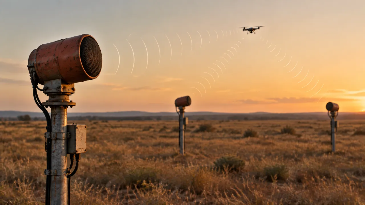
This is my continuation of the topic of sound location of air targets. In my previous article (Some challenges of drone acoustic location: why sound is not radio) I rashly promised to further analyze the possibilities of using the correlation-difference-rangefinding method of location. However, I soon became convinced that for a running engine drone This method will not work due to the regular structure of the sound.

Instead, I present to you another article analyzing passive sound location. The task appears to be non-trivial. I've outlined a solution.

Introduction

Drones-Drones have become widespread over the past decade weapons, which is revolutionizing military affairs before our very eyes. They are distinguished by their small size, low speed, and the ability to fly at extremely low altitudes while following terrain. This significantly complicates their detection by radar. Clearly, something needs to be developed to counter drones. In particular, it makes sense to try to detect and track them by the sound of their engines.

Sound ranging of air targets is the detection of flying aerial objects and the estimation of their coordinates and movement parameters based on the sound they emit. This is not a new concept; it will soon be 100 years old.

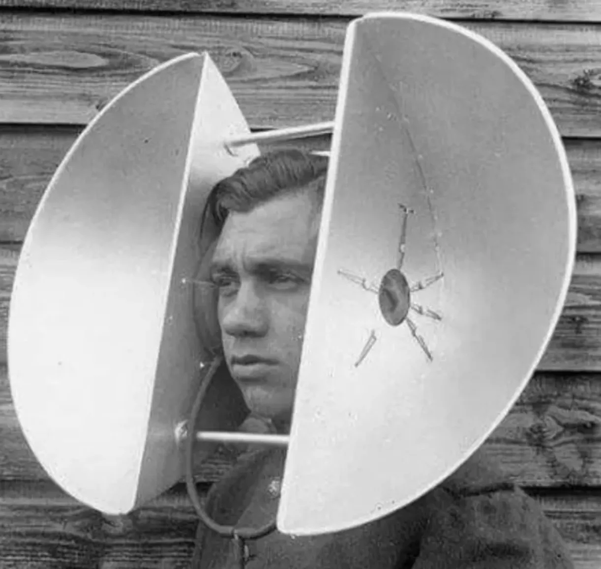
However, the author was unable to find a systematic analysis of the technical capabilities of sound ranging, particularly as it applies to drones, which have found widespread military use in the last decade. This article should, to some extent, fill this gap.

The sound of a drone's engine isn't particularly loud compared to an aircraft engine. Even a highly sensitive microphone can detect it at a range of no more than a few kilometers. We won't consider even more sensitive directional microphones here, as their use would require scanning the airspace using angular coordinates, significantly complicating the system. Therefore, we'll leave the angular (direction-finding) method of determining coordinates aside.

In passive radar, a correlation-based difference-ranging method for determining the coordinates of a noise jammer is well known. It is based on measuring the differences in signal propagation times to several receiving points located across the terrain. This difference is measured for each pair of receiving points using a cross-correlation function. Due to the purely random nature of the received jamming signals, this function has a single peak at the time delay corresponding to the difference in signal propagation times. This allows it to be measured. However, in the case of sound ranging, the signal has a significantly more regular, almost periodic, structure due to the operation of the air target's engine. Therefore, the cross-correlation function will have multiple peaks with a step size corresponding to the engine operating period. For example, at a frequency of thousands of revolutions per minute, the peaks of the sound correlation function will be spaced at intervals of tens of milliseconds, which corresponds to a spatial unambiguous interval of only a few meters, whereas we need thousands of meters. This precludes the use of the correlation-based difference-ranging method in the sound location of air targets.

In this article, we examine sound location using a single signal parameter—its frequency, observed over time from a single location or instantaneous frequency measurements taken simultaneously at multiple locations. Our method utilizes the Doppler effect, which causes the observed frequency to vary across different measurements. Based on these differences, we calculate the coordinates and velocity vector of an airborne target.

In considering the subject, we make a number of simplifying assumptions and accept several restrictions, namely:

• An aerial target (drone) on the observed section of the trajectory moves in a straight line at a constant speed.
  
• The sound of an aerial object propagates equally in all directions, having the same frequency spectrum.
  
• The detection system consists of a group of points dispersed in open areas, eliminating the possibility of reflected sounds. Interfering background sounds are virtually eliminated.
  
• Each receiving station has an omnidirectional microphone, a primary processing device for incoming audio signals, and data transmission facilities for the information consumers. The receiving station processes only audio by analyzing its frequency spectrum.
  
• A spectrum is characterized by a so-called characteristic frequency. This can be the frequency of the strongest harmonic (mode) or the spectrum width (average frequency or median). Therefore, a flying object can be considered to emit a monochromatic sound, the frequency of which may vary at different points due to the Doppler effect. During initial processing, the receiving station evaluates this frequency and, based on this frequency alone, can assess the remaining parameters of the aerial target.
  
• We consider the cases of a single receiving station and a system of cooperative stations that hear the sound of only a single air target.
  
• The stations are arranged so that several stations can simultaneously receive the sound of an airborne object. They can transmit the results of their primary processing to a central station for joint secondary processing with negligible latency.
  
• Simultaneous engagement of multiple aerial targets and measurement of bearings and/or other individual target characteristics requires separate consideration and is beyond the scope of our analysis.
  

It's well known that the detection range of an acoustic signal is limited to a few kilometers. Therefore, if high accuracy is required, acoustic location in the immediate vicinity of receiving points may be considered. From a tactical perspective, the Troops Defense This means that the sound location system can only serve short-range firepower as a target designation tool. It is desirable for the accuracy of determining the coordinates and velocity vector of a flying drone to be sufficient to allow targeting without additional search. Such a target could be an anti-aircraft machine gun or laser cannon located near the defended facility.

A sound ranging system can be effective as an early detection tool if the receiving station strip is sufficiently long and can be located at a significant distance from the defended facilities. Several such strips can be established at different points, complementing radar systems. The low cost of acoustic locators makes this possible.

Capabilities of a single reception center

For analysis, let's consider the circuit diagram Fig. 1This is a two-dimensional case. The coordinate system is chosen so that the target trajectory is parallel to the axis yThe velocity vector is directed toward decreasing this coordinate. The receiving point is located at the origin. In the following discussion, we will use capital letters to denote the sought-for quantities, and lowercase letters to denote known parameters.

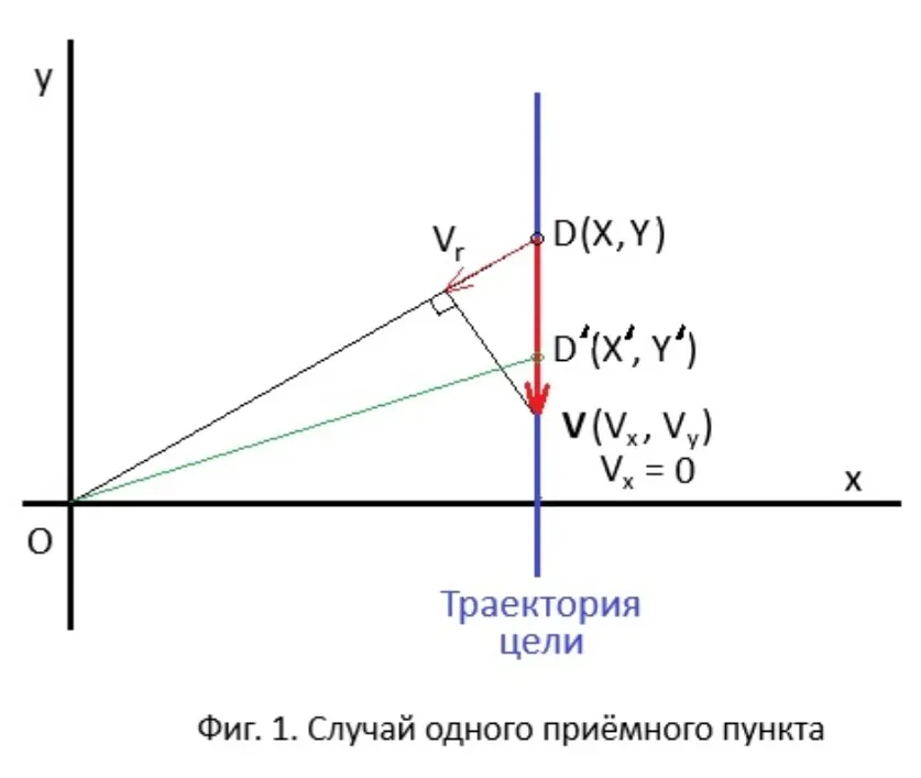
At the moment of receiving the sound signal the target was at the point D with coordinates (X, Y) and had a velocity vector V(V_x, V_y). At the moment when the sound reaches the receiving point, the target will fly some distance and end up at the point D'(X', Y'). Thus, the coordinates (X, Y) are apparent, and (X', Y') - real. Target speed V(V_x, V_y) along the entire trajectory, including at the actual point D' We consider it unchanged.

In the case of passive radar, the difference between the points D и D' Usually so small that it is neglected. In sound location, due to the relatively low speed of sound propagation, a correction is necessary. In the case of multi-location, these corrections differ for different receiving points. This is one of the peculiarities of sound location.

We want to estimate the parameters (X', Y', V_x, V_y) by the received sound with the observed frequency

f = F' + dF,

where F' - a characteristic frequency of sound unknown to us and dF - positive or negative correction, or Doppler frequency, which we also need to determine.

The latter can be calculated using the formula:

dF = 2 *Vr*F' / c,

where V_r - radial velocity of the target relative to the receiving point,
c - the speed of sound (about 340 m/s).

For example, for an air target flying straight towards the receiving point and with a characteristic sound frequency of 170 Hz and a speed of 50 m/s (like an airplane) An-2), we get:

dF = 2 * 50 * 170 / 340 = 50 Hz.

That is, the frequency of the perceived sound will be 220 Hz.

Since the characteristic frequency F' will be required for intermediate calculations, we will be forced to evaluate it too.

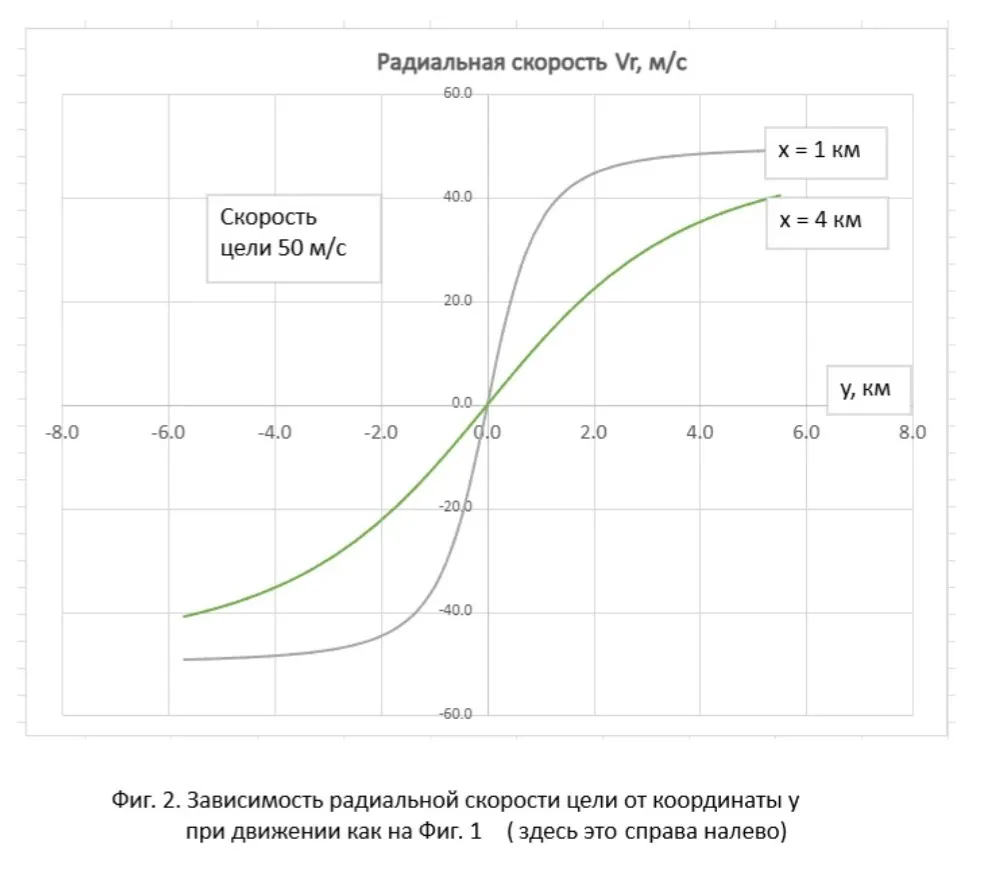
For Fig. 2 The graphs of the dependence of the radial velocity (and the Doppler frequency proportional to it) on the position of an air target are shown, assuming that it flies as shown in Fig. 1. That is, the coordinate y decreases, and looking at Fig. 2, we can assume that the target is moving from right to left. The Doppler frequency decreases monotonically. The steepness of the curve abeam the receiving station depends on the target's course parameter. x, i.e., its minimum distance from the receiving point. Two graphs are shown for the parameter 1 km and 4 km.

Doppler frequency unknown to us dF proportional to the radial velocity of the target Vr relative to the receiving point. It is "hidden" within the observed frequency f received audio signal. Frequency f carries information about all the parameters of the air target that interest us.

g(f) = (X', Y', V_x, V_y, F'),

Where g(.) is a function that connects these variables.

Thus, by measuring just one parameter f, in the two-dimensional case we want to estimate five unknowns. (In the three-dimensional case there will be seven unknowns, since Z и V_z).

To solve this problem, we have to measure the frequency f at least at five points along the trajectory, relying on the fact that due to the Doppler effect in changing f The parameters of the aerial target will become apparent. The curve in Fig. 2 shows that the Doppler frequency changes are more pronounced when the aerial target passes near the course parameter. This indicates that in the presence of frequency measurement errors at large distances, the Doppler effect may be excessively distorted by these errors. The best accuracy should be expected when the target passes overhead.

Calculation formulas and equations[/h3]
Here we are talking about expressions that connect the values ​​of the sought variables with the observed sound frequency.

Let i-th receiving point is located not at the origin, but at the point O_i, coordinates x_i, y_i which are known (i = 0, 1, ... , n-1). Our formulas work for both single-position and multi-position cases. The only difference is that in the second case, measurements are taken simultaneously, while in the first case, they are taken at different points in time. Oi does not depend on the index i, which is equal to zero.

The target course is arbitrary with a constant velocity vector V (V_x, V_y). In the single-position case, the true coordinates of the target change according to a linear law:

X'_i = X₀ + V_x* i * tau, (1)

Y'_i = Y₀ + V_y* i * tau, (2)

where tau is the time interval between measurements.

Since in the multi-position case the air target is observed by all points simultaneously, the true coordinates of the target do not depend on the index iAll other mathematical expressions are the same for both cases.

Let the apparent position of the target be a point D_i (X_i, Y_i); in general, it is different for each measurement, both for single-position and multi-position location. The distance to this point is determined by the formula:

The apparent coordinates included in it X_i, Y_i We have yet to determine.

Using the diagram in Fig. 1, we note that the radial velocity is the projection of the velocity vector onto the radius vector of the target. OiDiUsing the scalar product of vectors, one can obtain an expression for the radial velocity Fri. with i-m dimension:

Denominator is the length of the target radius vector O_iD_i, the numerator is the scalar product of this vector and the velocity vector V (V_x, V_y). The latter is the same for all measurements. We find it using the measured frequency. f_i:

f_i = F' + dF_i, (5)

where F' - characteristic frequency of sound and dF_i - Doppler frequency at i-m dimension.

The latter can be calculated using the formula:

dF_i = 2 * V_ri * F' / c, (6)

Where c - the speed of sound.

Knowing the speed of sound propagation, we will find the delay time

dt_i = d_i / c. (7)

This will allow you to extrapolate the apparent position of the target to the true one and find the actual coordinates of the target:

D'(X', Y') = D_i (X_i, Yi) and V (V_x, V_y) * dt. (8)

The last expression is vectorial and contains two scalar equations.

An attentive reader may have noticed that the given equations contain apparent coordinates X_i, Y_i. Knowing d_i, dtⁱ, they are determined by solving a system of equations.

Thus, for each of n sound frequency measurements f₀, f₁, ... , f_n-1 we have a set of formulas (1)-(8) that give us the function g_i(f_i) = (X', Y', V_x, V_y, d_i, dt_i, F') for i-th dimension. All these n sets form a system of equations that must be solved for unknown variables (X', Y', V_x, V_y, d_i, dt_i, F').

Since in the single-position case the measurements are made at known, but different, points in time, each of the variables X' и Y' will be presented by a set n values ​​corresponding to these moments in time. In this case, we evaluate the coordinate values ​​only for the last moment in time. Therefore, the system of equations will include the equations of motion of the observed aerial target (1), (2). In the multi-position case, these formulas will not exist.

Equations (3) and (4), however, are nonlinear, and the system of equations is unlikely to be solved analytically. This forces us to use numerical methods. This will require more the skill of applied mathematics than mathematical theory itself. The author leaves the demonstration of this skill to the reader.

Features of a multi-position system compared to a single-position system

A single-position passive sound ranging system is advantageous due to its extreme simplicity. The receiving station only needs to contain a sensitive omnidirectional microphone and simple electronic devices for amplifying the received signal, analyzing its spectrum, calculating target coordinates based on observations over a period of time (from a few to tens of seconds), and transmitting the coordinate and velocity estimates to the user.

A drawback of a single-position system is the assumption of a uniform, rectilinear target motion. If the target maneuvers, the accuracy of the calculations can be significantly reduced. If another similar aerial target flying at a similar speed appears in the detection zone during the observation period, this could confuse the calculations.

By complicating the location system, we can partially or completely eliminate the shortcomings of a single-position system. We trade off reduced time for increased spatial dimensions.

In the case of a multi-position system, the same mathematical formulas apply. The only difference is that for each sound frequency measurement, the coordinates of the receiving point x_i, y_i will have their own (i = 0, 1, ... , n-1). Also, when performing calculations, it should be kept in mind that when simultaneously receiving a sound signal at each point, the apparent positions of the target will correspond to different moments in time (Fig. 3). When calculating the true coordinates, this is taken into account by formula (8). With correct calculations, the extrapolated apparent positions of the target should coincide at the true point D'(X', Y').

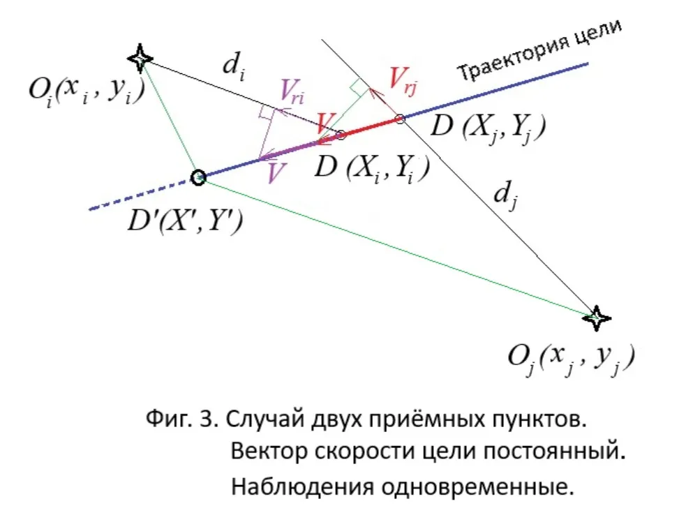
The single-position case differs only in that for each observation, the extrapolation of the apparent coordinates to the true point corresponding to the moment of the latter, (n-1)-th, observations are carried out according to a formula that takes into account the non-simultaneity of observations.

The obvious advantage of the multi-position method is that the full set of air target characteristics is determined almost instantly. "Almost" because during initial processing, some time is required to measure the spectrum of the sound signal and determine its characteristic frequency. That is, it's not exactly instantaneous. The lower the frequency of the sound, the longer it takes to evaluate its spectrum. In practice, this is the duration of 20-50 oscillation periods of the lowest tone. Therefore, for a frequency of 50 Hz, we spend up to one second determining the characteristic frequency. This delay must be taken into account when calculating the delay time included in formula (8).

Another advantage is that our assumption of uniform, rectilinear target motion is somewhat relaxed. The target only needs to maintain a constant velocity vector during the time it takes for the sound spectrum to be measured by all receiving stations. This means that it is possible to work against moderately maneuvering targets.

A disadvantage of a multi-position system is that we would need several receiving stations that could simultaneously and reliably detect the sound generated by an aerial target. Furthermore, the configuration of a minimal number of receiving stations is limited by the existence of blind spots. These are the positions of an aerial target when it is close to a straight line connecting a pair of receiving stations and is located on the same side of them. Since the Doppler frequency will be the same at these stations, our system of equations will not have a unique solution.

An interesting generalization could be the case where some receiving stations operate in single-position mode, while others operate in a distributed system, and their measurement results are combined. This can be useful when an aerial target is not observed by all stations simultaneously.

A possible approach to solving the acoustic location problem[/h3]
Let's clarify right away that the author does not yet have a ready-made method for solving the system of equations for passive sound location. This section presents only the basic ideas.

Equations (1)-(8) allow, given the configuration of receiving points and the parameters of the air target trajectory and the true frequency of its sound, to calculate the expected values ​​of the frequency of the received sound signal at each receiving point.

Below is an example for six receiver stations, evenly spaced around a circle with a radius of 2000 meters. The target coordinates, velocity vectors, and characteristic sound frequency at the time of measurement are shown above the table. Each row corresponds to one receiver station. The table lists the coordinates of the receiver stations, the distances to the apparent target positions, the target's radial velocities relative to these stations, the Doppler frequencies, and the observed sound frequencies.

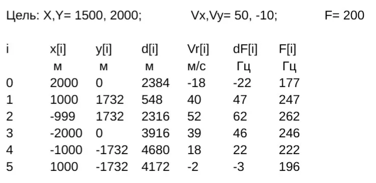
Such calculations are straightforward and can be used to generate data for testing a program for solving a sound-based location problem. That is, solving a problem that is the inverse of generating data like those shown in the table. However, developing such an algorithm is a non-trivial task. A possible approach to its solution is outlined below.

The solution can be found using the brute force method by trying various acceptable combinations of the desired parameters. X', Y', V_x, V_y, d_i, dt_i, F' and as a solution, select the combination that best satisfies the constraints imposed by formulas (1)-(8). Note that in the presence of n reception points of unknown independent variables will be 2*n + 5That is, for example, when n = 5 The solution must be searched for in a 15-dimensional space. The criterion could be the standard deviation of the observed sound frequencies from the frequencies calculated using formulas (1)–(8). However, such a simple solution search method would require an excessive number of trial calculations.

The range of acceptable values ​​of unknown parameters can be significantly reduced by using two groups of additional constraints arising from the specific features of the problem under consideration.

First group: all n the apparent coordinates of the target and its actual position must lie on the same line. This gives rise to 2*n linear equations.

The second group: the target velocity vectors, constructed from the radial velocity vectors relative to each pair of receiving points, must be equal. For example, in Fig. 3, the pair of vectors V_ri и V_rj allow you to calculate the target's velocity vector Vij. (The subscripts indicate the numbers of the reception points.) There are such pairs N = n*(n-1)/2. This gives rise to more N*(N - 1)/2 linear equations. When n = 5 we have 10 pairs and 45 equations.

This set of constraints significantly speeds up the search, making it easy to filter out unsuitable trial sets of values ​​for unknown variables and even conduct a directed search for a solution.

This class of problems in applied mathematics is called constraint satisfaction problems. This area has already been studied in considerable depth, and there are even software packages for languages Python и Java to solve them. The reader must learn to use these packages and represent the constraints in the required form.

However, it's worth cautioning against hasty steps. In our case, frequency measurements will be inaccurate due to interference. Therefore, some equations will not be satisfied simultaneously, and the solution to the problem will not converge completely. For example, not all velocity vectors will be absolutely identical, and the calculated frequency values ​​will not all be exactly equal to the measured ones. Thus, we arrive at the problem of satisfying fuzzy constraints. The interested reader is encouraged to explore the methods for solving this class of problems.

Conclusion

We've only examined the basic mathematical relationships between the measured frequency of a sound signal and the coordinates and motion parameters of the sound source. Two sets of questions remain unresolved for developing practical recommendations: technical and tactical.

Technical issues include the choice of a method for solving the system of equations, as well as ways to further refine the proposed mathematical model. Specifically, instead of a discrete method in the single-position case, the use of continuous-time equations and nonlinear filtering techniques suggests itself. It is also necessary to analyze the influence of a number of factors on the accuracy of estimating coordinates and the velocity vector, and develop appropriate recommendations. Since the entire game is played in terms of the Doppler frequency, it should be noted that accuracy will depend on the curvature of the curve in Fig. 2. The greater the curvature, the higher the accuracy. This influences the choice of timing for measurements. The selection of the characteristic frequency of the received sound also remains an open question. It would be desirable for the accuracy of the acoustic passive locator to allow target designation to short-range air defense weapons, which could immediately open fire without searching for a target.

Complex technical issues that remain to be explored include multipath propagation of sound waves, simultaneous engagement of multiple airborne targets, and the combined use of acoustic and other location methods. This places limitations on the tactical capabilities of the location method we've described.

Tactical issues relate to the study of options for constructing an acoustic location system at the lower level of the air defense system and methods for its combat use. Their solution depends on the resolution of technical issues, including the choice of configuration for a multi-position grouping of receiving stations. If an air target is too far away compared to the radius of the grouping, the sound frequencies received by different stations will have similar values, and the difference between them may be lost in measurement noise. Therefore, with an excessively dense grouping, solving the system of equations can lead to excessively large errors.

A cunning adversary could send us a very slow-flying balloon carrying a fairly powerful sound source. Due to the source's low speed, the observed frequency of this sound will be virtually identical at all receiving points. Under these conditions, the location methods described above will be ineffective. An adversary could also intentionally modulate the drone's engine speed to make frequency-based location difficult. These issues require separate consideration.

Thus, many interesting questions remain for further research.

Comments

[Maluck]

They are characterized by their small size, low speed, and ability to fly at extremely low altitudes while following terrain. This significantly complicates their detection by radar.

Acoustic detection systems are certainly good, but they are highly dependent on external factors - wind, air humidity, extraneous noise, etc.
The most effective detection method is radar, but as the author mentioned, this method has its limitations at low altitudes and in uneven terrain. The solution is simple: move the radars to higher altitudes and mount them on high-altitude UAVs, which could remain airborne for days at an altitude of 15-20 km and scan hundreds of kilometers in depth. This solves the problem of early detection of enemy UAVs flying in our direction.
China is currently testing the world's largest flying wing UAV, with a span of 52 meters, capable of flying for almost 24 hours at an altitude of over 20 kilometers. Why do you think they need it?

[Arhat109]

Well, to be pedantic, radar demonstrates its limitations not only in folded terrain and below the radio horizon, but also against wood-and-plastic "radio-transparent" solutions, especially for small FPV drones made from "stuff and crap." Acoustics here aren't a substitute, but a complement to other detection methods. With their drawbacks, of course. There's no single golden wunderwaffe, unfortunately.

[Same lech]

Quote: Maluck

The solution is simple: move the radars to a higher altitude and place them on high-altitude UAVs, which could remain in the air for days at an altitude of 15-20 km and scan an area hundreds of kilometers deep.

Airships need to be developed...they can carry stationary equipment weighing tens of tons.
One airship can accommodate several stations for different purposes: radar, acoustics, infrared scanning systems, and so on... the benefit is obvious... I don't understand what's stopping us from developing this area of ​​​​AEW&C.
By building a network of such airships deep within the country, we can plug the chronic holes in our air defenses through which NATO forces penetrate with their UAVs.

[Uncle lee]

In particular, it makes sense to try to detect and track them by the sound of the engine.

[Arhat109]

Since then, and perhaps even earlier, there have been at least 3 (three) ways to reduce the speed of sound inside a horn: filling with a porous material, filling with a medium with a low speed of sound (for example, krypton or SF6 gas), or a folded horn (see the topic about subwoofers).
At a sound speed of 120 m/s inside the horn, its input size (and length!) is reduced to 300 x 600 mm. )))

[VPKirillov]

the benefit is obvious
It would be good to clarify how you measure this benefit. For example, in rubles, the cost of developing a detection system given its specified combat effectiveness, including taking into account its resistance to enemy fire.
I've explored what's probably the cheapest approach. But it's too early to assess its combat effectiveness. Ensuring stability is relatively simple. A cluster of microphones in the reeds near a river isn't like a blimp sticking out like a fig. And the detection system itself should be built by combining several methods. There are many unresolved issues here.

[nikon7717]

Airships need to be developed...

A combined network of different detection methods is needed, in several layers.
It's already clear that in the future, UAVs could be used as terrorist weapons (launched from trucks and ships) within the country. Therefore, air defense/drone detection and control lines and rings are needed.
These lines, when used on a large scale, can and should be used to ensure traffic control and safety of civilian drones (they will also be regulated, it is expressly requested).
Accordingly, such lines will consist of radar, visual (machine vision), and acoustic surveillance systems. Observation points should preferably be located on tall structures (power lines, communication towers, chimneys), stationary aerostats, and on the ground.
As we can see, this is a large complex that needs to be integrated and provided with a large amount of different equipment. This is a fairly large production task for expanding/reforming the air defense network.

[VPKirillov]

Therefore, air defense/drone detection and control lines and rings are required.
At the same time, it is useful to assess what kind of increase in taxes and prices (including gasoline) our people are willing to tolerate.
We are already paying quite a lot for this non-war.

[Sarboz]

Quote: The same LYOKHA

One airship can accommodate several stations for different purposes: radar, acoustics, infrared scanning systems, and so on... the benefit is obvious... I don't understand what's stopping us from developing this area of ​​​​AEW&C.

The idea is viable. It needs to be developed further. There are objective limitations:
1. Vulnerability to air defense systems necessitates the use of stratospheric airships. Low temperatures there reduce the efficiency of batteries. Solar panels can only operate during the day.
2. Therefore, everything comes down to payload capacity. AWACS equipment is extremely energy-intensive and heavy. Ensuring 24/7 operation will require increasing the weight with large-area solar panels and high-capacity batteries.
3. Stabilizing the antenna will require a powerful automated motor control system. It's hard to imagine, but the weight will increase significantly. This isn't a quadcopter, after all.
It will be necessary to lift tons of equipment, the size of the airship will be enormous.

[Amateur]

Why 5? Azimuth, elevation, range. Changing these parameters will give the speed and direction of movement. That's all.

[Arhat109]

Another issue, as I understand it, is speed. Azimuth and target elevation are easily determined by phased array microphone algorithms, even with a 4x4 microphone. Speed ​​is determined by higher-harmonic barycenter-of-mass tracking algorithms. Range is more complicated; a decent separation is needed, as described in the article.

[nikon7717]

And speed, as I understand it. Azimuth and target elevation are easily determined by phased array microphone algorithms, even with a 4x4 microphone.

I believe the cited article emphasizes omnidirectional microphones, but range is far more important for detection, as it improves air defense response speed. Therefore, directional microphones are preferred. Although they are more expensive, when used with horns, they offer greater detection range and accuracy, and coverage increases at longer ranges. Directional microphones also need to be spaced apart to cover sectors. The end result is multiple positions and a method for determining direction and coordinates, as proposed by the author of the article.

[Arhat109]

The article says yes. I'm also in favor of directional microphones with a known pattern. In this case, spaced microphone positions, even in the same location, but aligned with the pattern's azimuth, allow for better performance.

[VPKirillov]

In the three-dimensional case, there will be seven unknowns. The target's Z and Vz will be added.
The acoustic receiver in my article doesn't measure the drone's range or angular coordinates. It only measures the motor's buzzing frequency.
More precisely, sound volume can be used to roughly estimate range, but this measurement is not suitable for targeting. It's only useful for detecting the drone's presence within the receiver's detection range.

[Arhat109]

The sound volume level depends on the distance, but it also depends greatly on... the wind direction, unfortunately.

[nikon7717]

The acoustic receiver in my article doesn't measure the drone's range or angular coordinates. It only measures the motor's buzzing frequency.

Besides the mandatory frequency, determining the UAV type is a straightforward matter. This isn't a particularly difficult task at the moment.
Phones have a similar feature that identifies songs and their authors by their melody. This would require additional training of existing AI models using different recordings, or the use of specialized programs with sets of reference samples, often from different UAVs. Essentially, a similar task is accomplished by marine buoys used to detect submarines, and by acoustic systems on ships and submarines. The experience and developments are there, but mass implementation is needed.

[Arhat109]

There's no need to drag in AI models everywhere. It's simpler. UAVs with internal combustion engines have a "fundamental tone" and multiple harmonics of the exhaust. Moreover, the power at the second harmonic is even higher than at the first. The situation with their propellers is roughly the same. It's quite sufficient to have two fundamental tones (exhaust and propeller) and the power distribution across the harmonics as a "portrait" of an ICE UAV. For copters with brushless motors and multiple propellers (quads, hexes, etc.), things are somewhat worse, but a similar profile is also quite possible.

[malyvalv]

It's unclear why all this complexity is necessary. The main thing is to detect the very fact of a UAV's flight at a specific point. A standard microphone on a cell tower can detect a UAV flying within a 2-3 km radius of its installation. That's the key. And given that UAVs fly at roughly the same speed, a pair of microphones perpendicular to each other can roughly determine their direction based on the rate of increase and decrease in volume. More is needed.
The X-hoolys have been installing microphones on all their cell phone towers for two years now and are now drawing maps with the flight paths of our Geraniums.

[Hexenmeister]

Difficulties? The author is trying to solve the problem of sufficiently accurate target designation for short-range air defense systems. And any "two microphones" will give the answer "Somewhere over there, beyond the river."

[malyvalv]

Close-in air defense systems with a 2-3 km range can see targets optically, just as well as hear them. They don't need acoustics. They are needed by mobile task forces and aircraft to know where to expect UAVs.

[Hexenmeister]

Especially if, without knowing where to expect it, it will rotate its optics a full 360 degrees, and there will be all sorts of things there: wires and poles, birds and trees, and, well, the data from the acoustics will not help aviation either.

[malyvalv]

That's why acoustics are needed to know approximately where to wait.

[Arhat109]

It's possible and long overdue. Acoustics aren't a very good choice for precise target acquisition. However, forward-facing microphones, as an early warning system for "something's flying around here somewhere," are quite useful, as they eliminate the need to fiddle with optics or thermal imagers.

[Sarboz]

Quote: Arhat109

It's possible and long overdue. Acoustics aren't a very good choice for precise target acquisition. However, forward-facing microphones, as an early warning system for "something's flying around here somewhere," are quite useful, as they eliminate the need to fiddle with optics or thermal imagers.

But there are already ready-made solutions, and proven applications in frontline areas. There's the compact "Ukho" system from NPO Alfa, which can detect a drone with an internal combustion engine at a range of 4-5 km and a copter at a range of 300-500 m. It's used in Belgorod and the Donetsk People's Republic. The bearing function is currently only implemented in the latest version.
Since May, BARS Kursk has been using the CBST complex with a neural network module.
Why can't it be implemented everywhere?

[Arhat109]

Unfortunately, I couldn't find anything definitive about these speakers other than various press releases from journalists. It's completely unclear whether these are individual high-quality microphones in each remote sensor with strong filtering algorithms, or a 700g phased array microphone, or a horn-loaded design (unlikely).
The range of a UAV with an internal combustion engine "up to 4-5 km" is completely unclear under what conditions and smacks heavily of marketing. Well, if that's under "ideal conditions," then it's not very impressive. The limit here is 15 km, based on signal attenuation at low frequencies of 75-500 Hz.
If you have any clear contacts for the developers, please send me a private message. I'd be happy to chat, as I've already minimized my design to a 240x240mm mouth with a hemisphere diameter just over 1 meter and a sound velocity in the horns of 117.6 m/s with a temperature range of -44.8°C and a frequency range of -6 dB from 85 Hz, excluding the horn gain (+23 dB). Expected range is down to 0 SPL.

[bk0010]

Quote: malyvalv

It is not clear what all these complications are for.

Issue the targeting instructions. The author did not address the complexities: environmental factors (wind, echo, extraneous noise), multiple UAVs, multiple engines on a single UAV, etc. were not taken into account.

[malyvalv]

Today, the capabilities of digital sound capture and computer analysis are simply incredible. It's even possible to imitate any voice without any problem. So these "difficulties" are simply a matter of computer sound analysis.

[bk0010]

Quote: malyvalv

So these "difficulties" are just a matter of computer sound analysis.

Yes, but "difficulties" in quotation marks are only used by those who won't have to deal with it. And the first question: are you sure the software development company will approve a list of imported components for you, including a chip with the required performance?

[malyvalv]

With sound, everything is tens of times simpler than with video, for example.

[Arhat109]

In a number of solutions, the "chip" is, for example, the Chinese equivalent of the STM32G473 - more than enough. )))

[Sarboz]

Quote: malyvalv

The X-hoolys have been installing microphones on all their cell phone towers for two years now and are now drawing maps with the flight paths of our Geraniums.

Just imagine, Kyivstar offered the opportunity to install acoustic sensors and related equipment on its towers free of charge. They also took on the maintenance.
But our "homegrown" mobile operator oligarchs don't want to do anything for free. The country's defense capability means nothing to them. They haven't disclosed the price they've set, but since the matter hasn't moved forward in Russia, the sums have proven prohibitive.
One cell tower was damaged today. Our cell phone bloodsuckers will only realize it when their sources of income are taken out by the dozens.

[Arhat109]

Are you sure they're "our own"? Back in 2003, I was trying to integrate a Quantum PBX into the city's communications system and suddenly discovered that all the towers were owned by the Canadian company Global One. I'm not sure how this works. Maybe "ours" isn't quite right?

[Sarboz]

Quote: Arhat109

Suddenly, I found out that... all the towers are the property of the Canadian Global One, I don't know how this... otherwise, maybe "ours" is not quite right?

I wouldn't be too surprised. Although a lot has changed since 2022. We don't notice everything, but there are changes. And it's not just McDonald's and Volkswagen. Sber, for example, which I often criticize. And yet, the share of foreign investors in it has decreased from 44% to 33%. The shares of the remaining investors from unfriendly countries are blocked; they can't sell them without our permission, and they can't withdraw dividends from the country.
The world is changing irreversibly. But parasites remain.

[VENOM]

The article is interesting and well-reasoned, but...

An aerial target (drone) on the observed section of the trajectory moves in a straight line at a constant speed.

и

Simultaneous operation against several air targets

Unfortunately, the restrictions are too restrictive. In any case, thanks to the author for a well-written and generally accessible presentation.

[VPKirillov]

Unfortunately, the restrictions are too strong.
This is a common approach in such studies. Without simplifying constraints, it is impossible to construct a mathematical model. Then, using this same model, they systematically study how relaxing certain constraints affects the algorithm's accuracy, and then refine it.
Without assumptions we get a random wandering in the dark.

[balabol]

A couple of questions on the topic.
1. In principle, similar issues are addressed in a different environment—water. After WWII, aerial acoustic systems stagnated, and target detection was relegated to radar. However, underwater confrontations provided numerous examples of working with sound in hydroacoustics. Both towed sonar stations and buoys—their technical implementations, and, most importantly, data processing methods—have advanced significantly. There are ready-made, proven solutions. I wonder if the author took them into account?
2. A common system for collecting, processing, and making decisions. What should it look like? A single microphone won't do much. Who, where, and how will process the data and make decisions?

[Arhat109]

Unfortunately, air isn't water. In water, the high speed of sound reduces the influence of interference, allowing for listening at a very considerable distance. Sound in air not only dissipates like a spherical wave and attenuates significantly with distance, but it's also mixed by wind and fluctuations. Hearing a drone with a base volume (at a distance of 1 meter) of 96 SPL is simply impossible beyond 15 km, even under ideal conditions. And German reconnaissance aircraft, as Gemini suggests, have a base volume of no more than 80 dB. Oops. 6 km is the dispersion limit under ideal conditions.
But, overall, the direction is correct - hydroacoustics has a bunch of different ready-made solutions.
2. Yeah. And then we run into Russian bureaucracy and a long line of officials with their prohibitive barriers and privately owned OCV towers. Unfortunately, no one will just turn this on anywhere.

[balabol]

Political will is needed. Mobile frequencies can be shut off, channel licenses can be revoked, and the towers will be handed over without a trace. There are power companies. There are tons of power poles, power, please, the data transmission network (Automated Electricity Monitoring and Metering System) is well-established. Acoustic sensors don't actually transmit that much information, not streaming video. The railway - power poles, data transmission system.

[Arhat109]

Is there one? Yeah. The commentary is too short... but the question isn't simple, judging by the situation with detection and interceptions. Especially in light of the latest decrees.

[balabol]

Yes. The ruling elite has this political will in spades. Without it, it's impossible to reach the pinnacle of power. The question is what are the priorities for its use and the plan of action. But such topics are for another thread.
This article discusses the specifics of sound propagation in various environments, processing systems, correlation functions, and AI training.

[Arhat109]

The details of sound propagation in different environments, as well as the processing systems, software, and other "complexities," have been known for a long time. Any AI will give you a vibecode in a couple of hours, and then throw out a bunch of questions like, "How do you plan to overcome this problem?"
Actually, not being an acoustician, I built my Hemdall-8km Navibcode using exactly this approach with three models in two weeks, or rather, in two pairs of weekends.
With a temperature range of -50 to +50°C and automatic temperature compensation, I determined the frequency response of a tricky horn, obtained the necessary formulas, methods for reducing the speed of sound and the horn's dimensions by almost 3 times, and even had to slow them down, otherwise, "Oh, this is a standard algorithm, if you want, I can give you the code for it in C, Python, or GO, it will be something like this..."
The advantage of phased microphone arrays is that they detect the signal direction based on the phase of the microphones in the array. A disadvantage is the difficulty of attenuating wind noise due to the high wind turbulence around the rectangular shape of the microphone array and the lack of a reference signal. The only way to suppress noise is mostly the microphones themselves.
A sector horn-based circular radar, on the other hand, aggressively subtracts noise and wind using a reference signal, allowing signals to be extracted 15-25 dB below the phased array. But:
A phased array (PAR) allows for software beamforming to track multiple targets, depending on the processing power of the processor. Unfortunately, the horn version cannot track many targets due to its low directional resolution.
Returning to "political will," a question as banal as a moo arises: if all this has long been known, AI algorithms are capable of providing reference materials of any complexity, then... what have our research institutes been doing for YEARS... or is there no "will" or is it in something else?

[stankow]

There's a terrible buzzing sound from coronal discharges on the power poles. Interference.

[balabol]

You don't necessarily need to use high-voltage lines. Active cancellation in the microphone is possible. Microphone directionality will also improve performance. You just need to play with the idea, find the pros and cons, try it out, do the math, and you'll see whether it's viable or not.

[virA]

This applies to high-voltage lines, starting at 220 kV. Such lines are of no use in this regard.
More interesting are the 35 and 110 kV lines, which cover fairly dense areas.

[stankow]

I meant 110 kV specifically. They're very noisy. Coronary discharges. Drive up, stop, and listen.

[VPKirillov]

Water has its own characteristics that air doesn't. Here are a few off the top of my head.
1. The speed of sound in water is five times higher than in air.
2. Target speeds in water are several times slower than in air. Combined with point 1, this means the Doppler effect in sonar is an order of magnitude lower than in air. It can even be neglected.
3. The frequencies of "useful" signals, such as propeller and airscrew noise, differ by tens of times. Combined with points 1 and 2, this creates an ambiguity of several meters in air due to the periodicity of cross-correlation, while in water, it can be hundreds or even thousands of meters. This makes the correlation-based differential ranging method impossible in air, but possible in water.
4. The aquatic environment has a noticeable vertical sound speed gradient. Due to the temperature stratification of the water, this gradient creates discontinuities in the gradient, leading to the formation of blind spots and channels for long-range sound propagation. This is not observed in air at the altitudes we are considering.
5. Sonar systems face the problem of clutter from the bottom. In the air, reflections from local objects can interfere. The common thread here is that reflections interfere. However, interference varies, and air defense systems can position receivers to reduce the impact. In sonar systems, if the target is a submarine, the commander's options are severely limited, and the bottom topography isn't always known in advance.
So there is some analogy, but there are too many differences.

[balabol]

Actually, my words should be understood as follows. Hydroacoustics and sonar have been more active over the past 40 years. Approaches to solving problems have been developed, and mathematical models for the operation of devices in heterogeneous environments have been created. If you look closely at what's been done there, you'll surely find a lot of useful information; there's no need to reinvent the wheel.
If you think you have processed this array of information in full, then great, I envy you.

[Alexander Bezfamilnuy]

What can be said with certainty right away is that with this approach, practical implementation will not happen anytime soon.
And it is quite possible that it will no longer be relevant.
"Single omnidirectional microphone"... Wind and other joys of real life... Try recording sound in the wind.
There are four microphones. At each station. Quite ordinary ones. With a microphone amplifier at each. It's simple. A simple board the size of a fingernail.
Each microphone has a horn. This is even simpler. For example, an aluminum or plastic plate with a soft, porous, sound-absorbing coating on the outer surface. A simple board like an ESP32 can be used for initial data analysis, but four channels, one in the center, is better.
Four channels will already give an approximate direction and speed.
Let me emphasize – APPROXIMATE. We don't really need EXACT parameters. This is a detection network, NOT a targeting one.
Its task is to monitor the space 24/7/365 and transmit data to the processing center.
For example, cell phone towers. They have power and transmission capabilities. I don't know how densely they're spread across the area.
Agorithm. Such and such a point (a specific place on the map), approximate destination, approximate direction.
The neighboring station also hears, giving the center more computing power and increased accuracy.
The target moves from point to point, and the center thus plots a route. Approximate.
Precision will be needed for weapons of destruction. For example, a light aircraft with small-caliber machine guns. Even a .22LR.
One target, several, a swarm of targets... This is a task for a machining center. NOT for every point.
Calibration and training of the system.
1. Turned on.
2. For example, they launched a light aircraft from point A to point B.
The system recorded, analyzed, and calculated the coefficients.
3. They sent several light aircraft along a winding route with varying altitude...
Well, etc.
And the author of the article can sit at the terminal communicating with the district analysis center and practice mathematical calculations as much as he likes, tweaking the program as needed. Tweak it, train it.
By the way, this is where AI can come in very handy.
Let me repeat. The importance of this system is greater. It's a way to also detect counterintelligence in the event of a major conflict.

[Arhat109]

That's right. And the circular horn version doesn't even require any adjustment. It can also subtract wind signals from opposing horns and apply NMLS algorithms or even more advanced ones.
But NO ONE needs this! I already posted my Heimdal-8km – a circular radar design with 12 30* sectors and a theoretical detection range of 8-10 km.
Deaf! Either there are no "acoustic specialists" here, or no one needs it.
Special respect to the author for taking on the task of writing a whole series of articles on this topic.

[Alexander Bezfamilnuy]

I'll also add something that I didn't have time to correct/add right away.
A processing center with a distributed network of microphone points is the only configuration that is capable of accomplishing the task in any way.
A typical PC should be powerful enough for several dozen microphone stations, meaning it should cover a certain area. The author, however, is persistently trying to improve accuracy and is relying on a limited number of microphones. This is a dead end.
A single microphone will produce nothing but noise, even in a gentle breeze. I'd advise the author to try recording audio with the same smartphone, even in gentle wind.
Horn quadruple dots, oriented to the cardinal points, will immediately provide direction, speed, and possible target parameters.
And the author apparently doesn't understand that high precision isn't necessary. A few hundred meters, give or take. Specific detection is the responsibility of the mobile team.
The designer's experience tells us that complex algorithms at the start of an idea are precisely the way to bury the project.

Quote: Arhat109

Deaf! Either there are no "acoustic specialists" here, or no one needs it.

I have the same feeling. He's not promising any profit, so he's not interested... And the government seems to be in a hurry. Vitek and his son-in-law are showing up, and the elections are coming soon...
I really want to be wrong. And it's entirely possible that I'm wrong in this assumption. This isn't the kind of topic that gets extensive coverage in open sources.
Moreover, I have doubts: am I working for the enemy by publishing such things here?
And I probably would have refrained if similar things hadn't already been heard among Ukrainian radio amateurs at the very beginning of their use of the Geraniums. For example, with the Radiodinosaur.

[balabol]

This is the eternal struggle in distributed systems. Should we complicate the peripherals (sensors) and simplify the central processing unit, or should we create many primitive peripheral devices and concentrate everything in the center? A hierarchical system is possible: peripherals, nodes, center. In a practical sense, we need to calculate. Ideologically, of course, we need to increase the coverage area by saturating it with sensors and obtaining data redundancy, thereby increasing the accuracy and stability of the system as a whole. (I would have started the project this way if someone had asked me to.) ).

[Alexander Bezfamilnuy]

Quote: balabol

It's an eternal struggle in distributed systems.

Considering the size of the country and the length of the possible perimeter that needs to be covered, I think the issue should be addressed solely by reducing the cost of sensors.

[Arhat109]

There's no need to cover the entire perimeter. The range of acoustics is limited by physics and doesn't exceed 10-15 km. It's these 5-10-15 km that should be covered by an early warning system for target air defense, especially in areas where radar can't cope due to the radio horizon, terrain deficiencies, and radar background (highways with lots of moving traffic).
So, speaking of profits: quantity restores profitability for a business, even with a small per-unit margin. What's that margin? Phased array microphones are currently offered at prices in the region of 300-100 rubles. A product consists of 32, 64, or 128 microphones, each priced at 200-200 rubles. The rest is hardware and software with a DSP processor (5-10 rubles). Horn-based options will cost about the same, and with similar delivery costs... but apparently 8-10 times that is "a bit low."

[Alexander Bezfamilnuy]

There is no need to cover the entire perimeter.

Only at the first stage. Only in the most probable directions.
And then it got worse. Actually, it got worse. Those same drones all over St. Petersburg.
And given the likelihood of a global strike with a mass of tomahawks and other scalps...
The entire European border. The entire south of the country. The Far East.
I'm afraid this unstable world will last a long time. Of course, you can give up, which is what the government will likely do.
Targeted air defense? What's the point? By the time a mobile task force with anti-aircraft weapons arrives, a light interceptor will arrive... Once they're detected, it's too late to intercept. Only distant outposts can offer any chance of interception.

[Arhat109]

And this thing is useless against Tomahawks, except perhaps as a border weapon. 800 km/h is a significant factor for acoustics. By the time it identifies a target (even from 40 km away), the Tomahawk will have covered 80% of that distance, just like any other high-speed missile.

[Alexander Bezfamilnuy]

Why is it useless? There's a strike coming. The most reliable way to determine where the wave is coming from is precisely at the border.

[VPKirillov]

You and a number of other commentators are clearly stuck in outdated notions about a future air defense system. Mobile groups will soon be gone because they won't be able to cope.
In the coming years, we'll see clouds and swarms of drones attacking us. We can't keep up with all our mobile units. I see a possible solution for close-in air defense in the development of automatic, rapid-fire weapons. This isn't a new idea—automatic firing devices were installed on the infamous Berlin Wall against the Germans trying to breach it. I hope this inhumane method can be used to defend our facilities, such as oil refineries and air defense missile systems, from drones. That is, for a humane purpose. To achieve this, we need to develop means of detecting and targeting incoming drones with sufficient accuracy. The accuracy of the methods I've described here remains to be determined.

[balabol]

Great, we've already moved on to money. That's the most exciting part of any project. But first, let's go back to the beginning of the story (cleverly said).
The technical specifications begin with the role of the system being developed in the overall air defense system. Who is the customer? The class of objects being protected, the scope of use, who provides data to this system, and to whom it transmits its data. Communication interfaces. Who uses its data. The system structure, the number of system elements, and the GOST standards the system and individual elements must comply with. The Ministry of Defense will pay only for a complete system that meets GOST standards and regulations and will interface with the overall information system, as well as for service, warranties, support, etc.
I assume you've worked with the Ministry of Defense and understand their software certification requirements, have passed the SP and SI, and are familiar with the information transfer requirements, etc. Prices are objectively increasing exponentially.

[Alexander Bezfamilnuy]

Yes, the questions are important.
Both the solution and the main obstacle sound the same: political will. Or the lack thereof.
For some reason, it is not customary to talk about one of the main reasons for the Great Victory.
Bureaucracy was completely eliminated. Direct control of industry. Plus personal responsibility.
Do you really think that compliance with GOSTs, regulations, and other waste paper is more important than the country's survival?
But in the absence of will, all these tugaments are an excellent excuse to do nothing. On completely legal grounds.

[balabol]

Bureaucracy was COMPLETELY eliminated. - incorrect statement.
It's not that simple. I understand what you wanted to say, but!
Bureaucracy is a system of exercising power through a specialized administrative apparatus. So, in this sense, bureaucracy remains, but it has been modernized. New structures have emerged.
The highest governing bodies were created at the beginning of the Great Patriotic War.
The State Defense Committee (GKO) was established on June 30, 1941, by a joint resolution of the Presidium of the Supreme Soviet of the USSR, the Council of People's Commissars of the USSR, and the Central Committee of the All-Union Communist Party (Bolsheviks). The General Command Headquarters was established on June 23, 1941, by a resolution of the Council of People's Commissars of the USSR and the Central Committee of the All-Union Communist Party (Bolsheviks) to provide strategic leadership to the armed forces. It was initially headed by Marshal S.K. Timoshenko, the People's Commissar of Defense. On July 10, 1941, by a resolution of the GKO, it was transformed into the Supreme Command Headquarters.
The Evacuation Council was established on June 24, 1941, by a decree of the Central Committee of the All-Union Communist Party (Bolsheviks) and the Council of People's Commissars of the USSR to coordinate the relocation of population, institutions, military, and material resources from threatened areas to the rear. Specialized departments were also established under the Council of People's Commissars, such as the Department for the Evacuation of the Population (September 1941). 
Specialized committees under the State Defense Committee
To solve specific problems, specialized committees and commissions were created under the State Defense Committee, for example:
* Transport Committee (formed in September 1942); 
* Committee for the Evacuation of Food and Industrial Goods (October 1941); 
* Operational Bureau of the State Defense Committee (December 1942) to control the work of the People's Commissariats of Defense
These bodies made it possible to mobilize the country's resources to repel the enemy and establish clear interaction between the front and the rear.
Do you really think that compliance with GOSTs, regulations, and other waste paper is more important than the country's survival?
Well, first of all, we're reviewing the existing system. I've described how it all works within the official project. Regarding the rules and GOSTs, I have a question for you: will we be checking the equipment for hostile implants, software for malware, and maintaining communication with the external control loop? If so, we'll have to work within the GOSTs.

[Alexander Bezfamilnuy]

If yes, then you will have to work in accordance with GOST standards.

If there are calm decades ahead, then yes.
But if "it was necessary yesterday," then only political will can force bureaucratic structures to take a sober look at the requirements of the extremely extensive, sometimes contradictory legislation, state standards, rules, regulations, and so on, taking into account the priorities of the tasks.
I speak as a former safety engineer. I've encountered this in practice.
Moreover, I can say with a high degree of probability that if FULL compliance with the entire spectrum of regulatory documents is required, NOT A SINGLE enterprise in the country will pass.
The caring lawmakers and rulemakers have produced far too many different things. Naturally, "for improvement, provision, and perfection."

Bureaucracy is a system of exercising power with the help of a special administrative apparatus.

You and I have slightly different meanings. Bureaucracy in the sense of plans, reports, approvals.
Of course, something remained, but the main thing became expediency.
I don’t know if you’ve ever had to draw up “3-year development plans,” for example.
I had to calculate inflation myself. For some reason. And they could approve some portions, or they could arbitrarily cut them, as the higher-ups saw fit. They could give crazy amounts of money for things that were completely unnecessary and not spend it on what was needed. And certifications and the like are a whole other story.
I'm talking about this bureaucracy.

[VPKirillov]

Thank you for your comment.
I'd like to clarify something. In my calculations, I left out the description of the receiving points and the use of additional measurements like angles and distances in a separate section. If you want to install four microphones with 360-degree horns at one point, go ahead. By summing the signals they receive, we get what I called an "omnidirectional microphone." Because I was only interested in what could be extracted from this sum for location. There's no point in multiplying entities when even in such a simplified configuration, everything isn't so obvious. This needs to be fully understood. For example, the accuracy of determining the target's coordinates and velocity. This is a separate scientific and engineering problem.
I also suggest everyone (not just you) avoid mentioning AI and using terms like "easy" without showing what and how AI can do it, what kind of AI it is, and how easy it all is.

[Arhat109]

Let me explain. AI is a vast collection of all of humanity's knowledge in a training dataset. In fact, this knowledge turned out to be vastly insufficient for learning tasks; in fact, it's not as abundant as we'd like. A drawback of AI models, even the latest Transformers, is the generation of plausible nonsense. This occurs when a query the model is asked for doesn't have an answer in its training dataset, and it picks up something "similar" (and a model is obliged to answer any query!), since it has no "understanding" at all. Therefore, the only useful application of AI is as a "knowledge library." Ask for information found in textbooks, dissertations, and other collections that would take a lifetime or more to find. Moreover, before making a query, it must explicitly allow the "I don't know" answer—that is, prohibit the generation of nonsense. Models with web search can also provide links to the answering material. These links must be verified for validity. With a certain skill, getting the knowledge you need from it is truly easy and much simpler than browsing libraries or Googling. In fact, it actually does all the searching itself, even if it's not shown in the search results.
If I were you, I wouldn't "build a theory" (there are plenty of them already built) but would rather be puzzled by the query about what already exists and what they allow us to solve in matters of signal location.
But overall, yes. I often see attempts to shift the search for solutions to a delusional model; sometimes it's even funny. It's worse when it's done by a "hand-waving" person... the joke about Khrushchev's landing on the Sun is nothing special. )))

[VPKirillov]

I'd like to modestly note that I was the first person at the Ministry of Defense to defend a doctoral dissertation in AI, in 1991. Therefore, I use this term cautiously myself and am suspicious of texts that use it without specifying which part of AI the author is referring to and how it is specifically used. It's being used inappropriately everywhere these days. And this is a very broad field. For example, computer vision with scene recognition, speech recognition with meaning comprehension, the synthesis of chemical compounds based on their text descriptions, and much more. It's simply too much to list.

[Arhat109]

It's worse when these nonsense generators are used by "effective managers." And they are. The same mess in Iran was generated by the AI ​​Cloud, which the Pentagon consults. The results are obvious, as they say.
And yes, the AI ​​of the 90s was "expert systems," but today's is something entirely different. A modern transformer is a pure nonsense generator, its main task being to derive the next token (not even a word, often a syllable!) by running the entire previous context (from the very first query, including its own nonsense!) through the dataset each time.
You can't "generate" anything there, only requests like in an online library.

[salawat1980]

Quote: Aleksandr Bezfamilnuy

There is no need to cover the entire perimeter.

Only at the first stage. Only in the most probable directions.
And then it got worse. Actually, it got worse. Those same drones all over St. Petersburg.
And given the likelihood of a global strike with a mass of tomahawks and other scalps...
The entire European border. The entire south of the country. The Far East.
I'm afraid this unstable world will last a long time. Of course, you can give up, which is what the government will likely do.
Targeted air defense? What's the point? By the time a mobile task force with anti-aircraft weapons arrives, a light interceptor will arrive... Once they're detected, it's too late to intercept. Only distant outposts can offer any chance of interception.

Firstly, the sound can be used to determine the azimuth and elevation for launching a drone. This accuracy is more than sufficient. Secondly, as correctly indicated, a tetrahedron (pyramid) with horn microphones (ordinary 5 cm cones) is already a phased antenna array. Wind and other problems are solved. Simply cover the horn with acoustic fabric. Other interference is irrelevant to us, since a fast Fourier transform/cosine transform is performed anyway. We are initially working with sound, which is the drone. Obviously, no ESP32 will suffice for this task. You need a JETSON or a decent PC with a graphics card. The ESP32 cannot perform phase distribution in real time. Filtering requires converting the sound into a sum of sine waves and then selecting only the drone's signal. Your simple equipment will not be able to transmit packets to the center without delay. Ping your WiFi router and multiply the ping by the speed of sound. The difference in pings will be an error. This will prevent you from aiming or aiming. The distance error will be too large.

[Arhat109]

It is obvious that no ESP32 will be enough for this task.

But here you're completely wrong. It's perfectly sufficient for digitizing 12 or more channels, even with oversampling to 15 bits from the existing 12. A sampling frequency of 6 kHz after oversampling is perfectly sufficient for the 80-3000 Hz range, and that's all you need. And STMs come in a wide variety, from 48 MHz to 600 MHz clock rates. It's perfectly adequate.

Your basic equipment won't be able to transmit packets to the center without delays. Ping your WiFi router and multiply the ping by the speed of sound. The difference in pings will be an error. This will make it impossible to aim or target. The distance error will be too large.

You're right about that. Any acoustic radar has a significant delay, which precludes accurate and timely target acquisition. And the more we want to average the FFT, the greater the delay.

[VPKirillov]

"Any acoustic radar has a delay, and a fairly significant one, which precludes accurate and prompt target designation."
It seems you didn't read my article carefully. I focused specifically on eliminating the effects of this delay, and I consider it an element of innovation. To achieve this, I distinguish between the apparent and true coordinates of an aerial target.

[VPKirillov]

I ran into an editing time limit. Here's my revised post.
--------------------------
"Any acoustic radar has a delay, and a fairly significant one, which excludes accurate and prompt target designation."
It seems you didn't read my article carefully. I paid special attention to eliminating the impact of this delay, and I consider this an element of novelty. For this purpose, I distinguish apparent и true air target coordinates.
Ideally, using my equations, the target's coordinates and velocity vector can be determined with absolute precision and instantaneously. I demonstrated this using 9th-grade mathematics.
The next step is to investigate the impact of deviations from the assumptions I've made and frequency measurement errors at receiving stations. This will allow us to evaluate the real capabilities of the proposed Doppler sound location method. This would require the work of a couple of PhD theses. Only after this research is completed will it be possible to discuss practical implementation.

[Arhat109]

Unfortunately, all your math boils down to the speed of sound. By the time the signal reaches the receiving sensor, the target is moving at its own speed "somewhere," not flying "straight and steady," alas. And the target's sound doesn't spread evenly across a sphere. The limiting case is supersonic flight, and no math will help here, because you'll only hear it after you've actually passed—"later."

[VPKirillov]

Unfortunately, all your mathematics comes down to the speed of sound.
My math (at the 9th grade level) doesn’t rely on the speed of sound, but takes it into account and uses it explicitly.
To constructively criticize the restrictions I've adopted, I need to measure how burdensome they are. This is a topic for future research.
At a qualitative level, I can make the following assessments.
A drone typically flies in a straight line near the impact site. For the Doppler method described above to work, the drone only needs to fly in this direction for 5-10 seconds. Therefore, the assumption of uniform, rectilinear motion seems reasonable.
Regarding supersonic speeds. The current challenge is combating drones flying at altitudes of up to 100 meters, where radar systems, if they have any visibility, do so only intermittently. And at such altitudes, it's impossible to ensure safe flight for a drone flying at supersonic speeds. "Our" drones are all slow. Radars can handle supersonic drones flying at altitudes of 300 meters and above.

[Arhat109]

Yes. I'm talking about those 5-10 seconds. For a Tomahawk, that's up to 3 (three!) kilometers. And yes, a drone can fly in front of an object however it wants, including anti-missile maneuvers and various "climbs." But the approach trajectory is determined by mapping, the underlying surface, and the flight mission. I'm talking about ultra-long-range drones attacking civilian infrastructure. On the front lines, acoustics essentially have nothing to do.
Tomahawks and modern cruise missiles have an "operating altitude range" of 5 to 50 meters. 100 meters is prohibitively high. "Ours" may be, but the Geran-5 claims otherwise.

[VPKirillov]

from 5 to 50 meters
This is above the water surface.
Over a city like Moscow, a drone can fly along avenues at a level just below the rooftops. This should be a source of great concern for the commander of the Moscow Air Defense Zone.
This will be "our" subsonic drone. Very sub-. Ours, I mean—a target for sonar location.

[Arhat109]

No. That's already over land too. Recognition systems were already achieving 20-30 frames per second in 2023, even on the Jetson X-Warrior, when they were writing their ballistic calculator. And this is just... a "toy," for the most part.

[salawat1980]

I wasn't talking about digitization, but about the Fourier transform and phase comparison. You mentioned this in the second half. It seems like an FFT alone won't do here. The larger the FFT window, the more accurate the calculations, the greater the latency, and the further the target can shift. I can't argue with you on that. Besides, if you have the noise of a battlefield, the noise of wires... Neither the ESP32 nor the Orange Pi 5 can keep up. How are you going to transmit the signal to the server without latency? The worst part is that even over UDP, it can change.

[Arhat109]

Quote: salawat1980

How are you going to transmit the signal to the server without latency? The worst part is that even over UDP, it can change.

It depends on what you're talking about. The signal travels to the server much faster than sound. It can be transmitted over a telephone line (a twisted pair cable is a good option), fiber optics, satellite, radio, Wi-Fi, using standard or proprietary protocols. Even with a laser pointer (we used a mesh between the balconies)!

Quote: salawat1980

Also, if you have a battle noise, wire noise... Neither the ESP32 nor the Orange Pi 5 can keep up.

Again, it depends on the task and the acoustic reception methods. Noise from wires, microphones, and other electronics can be eliminated using horn systems with geometric gain higher than this noise. This also improves reception directionality. The rumble of combat can be processed by an op amp with automatic gain control. The rise time of these amplifiers is insane, even for mediocre op amps like the MC33079 (4-piece package). And then again, we need completely different algorithms for UAV detection than for artillery shell direction finding. What's good for a shell direction finder is bad for UAV detection, and vice versa. These are different systems.
Neither the ESP32 nor the Raspberry Pi are suitable as sensor data acquisition controllers, not because of their performance, but because they lack the required number of ADC channels with the required speed and bit depth. This means we need to invest in an external ADC kit, which significantly increases the overall cost of the device: board layout, number of enclosures, and size.
The STM32G473 and its analogs, as well as newer devices, are particularly good because they have 4-5 simultaneous ADC sampling units, each with 4-5-8 multiplexed channels. This gives a total of up to 42 channels with high sampling speed—something like a 60 MHz ADC clock and 4 million 12-bit samples per second. Oversampling by 64 samples yields 15 bits. That's already sufficient.
For example, my 12-sector Heimdall-8km is four ADC blocks simultaneously, multiplexing three channels each and oversampling up to 15 bits (64 samples). The total is 4msps / 3 / 64 = 20.8ksps – a sampling rate of 20.8 thousand samples per second. Note that all this is achieved without any involvement of the microcontroller itself, purely by hardware, using interrupts and direct memory access.
20.8k measurements allow us to use this frequency as the upper frequency of the device, but we don't need a sink. Dividing /256 instead of /64 yields 16 bits from the ADC and an upper frequency of about 5 kHz. More than enough. You can even use a pair of four MC33079 op amps to create not only an AGC unit but also a second- or even third-order bandpass filter for 80-5000 Hz, leaving one op amp solely for matching the ADC input.
Something like that. Note that the processor itself isn't really involved in this scheme. At 120-160 MHz, it's just right for NMLS, FFT512 (1024, and again, no more is needed), and averaging with result search.
It can't transmit, it doesn't really have anything to transmit with, although... it has a ton of SPI and again it's hardware-based.
Where does he "fail"?
P.S. There's a built-in float, but it's mostly unnecessary. ADC integer calculations are often simpler and faster.

[VPKirillov]

Firstly, the sound can be used to determine the azimuth and elevation for launching the drone.
The devil is in the details.
What you wrote refers to the direction-finding method of sound location. I deliberately excluded its use in my article, aiming to analyze the potential of the purely Doppler method. Combining it with direction-finding would dramatically reduce the amount of calculations. And perhaps improve accuracy. Or perhaps not improve it at all. This question awaits its research.

[agond]

Quote: salawat1980

We don't care about the rest of the interference, since we'll be performing a fast Fourier transform/cosine transform anyway. We're working with sound, which is a drone. Obviously, no ESP32 is sufficient for this task. You'll need JETSON or a decent PC with a graphics card. The ESP32 can't perform real-time phase dispersion. For filtering, we need to convert the sound into a sum of sine waves and then isolate only the drone. Your simple equipment won't be able to transmit packets to the center without delay. Ping your WiFi router and multiply the ping by the speed of sound. The difference in pings will be an error. This will prevent you from aiming or targeting. The range error will be too large.

Filtering and amplifying all the sounds that came to those microphones is like picking through a pile of garbage, a dubious and thankless task, you need a special microphone (or
group of microphones) which is sensitive only to the flat front of acoustic waves from distant sound sources; waves from nearby sound sources have a spherical front and therefore should not be perceived by the microphone.

[Arhat109]

This is typical work for DSP algorithms and special processors.

[VPKirillov]

I just found a scientific publication on passive radar that uses a combination of differential ranging and Doppler methods. Taking the Doppler effect into account dramatically improves the radar's capabilities. The authors also assessed the accuracy of their method. It was shown that it is possible to significantly improve resolution, reducing the interference of other airborne targets.
http://jre.cplire.ru/jre/sep17/13/text.pdf
Something similar could be done for sound location.

[Arhat109]

Excellent material, thank you. It's a shame I can only give one upvote.

[salawat1980]

Quote: Arhat109

This is typical work for DSP algorithms and special processors.

The special algorithm needs to process a lot of values. And it takes time for the microphone to produce these many values. A combination of the Doppler approach and passive array direction finding is the obvious choice. Beamforming itself is a filter. The author of the article beat me to it, even providing a link. Thank you very much for practicing this and explaining to people how it works.

[Arhat109]

You're welcome. I'm not an acoustician, unfortunately. I've been a pogromist since about 1979. )))

P.S. I'll add another point. I've got a strong feeling that the military is still using Setunya and BESM-6, with its once-groundbreaking megaflops. Only now, microcontrollers, with negligible power consumption, are capable of delivering hundreds of megaflops, all on a board measuring just 2-4 cm².